
Tensorflow
- 2015년 11월 출시
- 구글 브레인 팀에서 심층 신경망을 위해 개발한 강력한 오픈소스 소프트웨어 라이브러리.
- 자동 미분, CPU/GPU 옵션 지원, pre-trained model 등 지원.
- Python, C++, JAVA, R, Go 등 주요 언어 작업 가능.
- Keras가 Tensorflow에 통합
- Keras는 마이크로소프트 CNTK, AMAZON mxnet, 티아노 등 여러 딥러닝 엔진에 통합 될 수 있다.
- 쉬운 모델 배치 및 생사느 시각화 기능, 커뮤니티 활성화 등의 장점.
- 2.0 버전 부터 keras 단순 코딩 사용, 직관적 프로그래밍 적용.
▶ 설치
!pip install tensorflowimport tensorflow as tftf.version.VERSION
import sys
print(sys.version)
# 3.9.12 (main, Apr 5 2022, 01:53:17)
# [Clang 12.0.0 ]
▶ 신경망을 위한 데이터 표현
스칼라 (0D 텐서)
넘파이에서는 float32, float64 타입의 숫자가 스칼라 텐서.
▶ Data load
from tensorflow import keras
from tensorflow.keras.datasets import mnist
(train_images, train_labels), (test_images, test_labels) = mnist.load_data()print(train_images.ndim)
print(train_images.shape) # 데이터수, 행, 열
print(train_images.dtype)
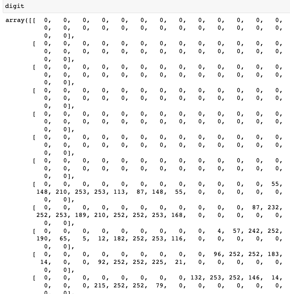
digit = train_images[4]
plt.imshow(digit, cmap=plt.cm.binary)
plt.show()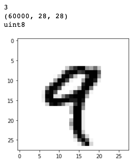
▶ digit을 확인하여 각 위치의 색의 밝기 값을 확인
▶ Slicing
(90, 28, 28) 출력
my_slice = train_images[10:100]
print(my_slice.shape)

# 자세한 표기법
my_slice = train_images[10:100, :, :]
my_slice.shape

my_slice = train_images[10:100, 0:28, 0:28]
my_slice.shape


# (90, 28, 28)
▷ 부분 출력
my_slice = train_images[:, 14:, 14:]
plt.imshow(my_slice[4], cmap=plt.cm.binary)
plt.show()
my_slice = train_images[:, :-7, :-7]
plt.imshow(my_slice[4], cmap=plt.cm.binary)
plt.show()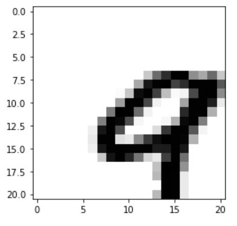
▶ 배치 데이터
batch1 = train_images[:128]
batch2 = train_images[128:256]

# n번째 batch
n = 3
batch3 = train_images[128 * n : 128 * (n+1)]
vector = coulums
▶ 텐서의 실제 사례
- Vector Data : (samples, features) 크기의 2D 텐서.
- 시계열 데이터 또는 시퀀스 데이터 : (samples, timesteps ,features) 크기의 3D 텐서.
- 이미지 : (samples, timesteps ,features, channels) 또는 (samples, timesteps ,features, width) 크기의 4D 텐서.
- 동영상 : (samples, frames ,timesteps ,features, channels) 또는 (samples, frames, channels, height, width) 크기의 5D 텐서.
▶ Verctor DATA
- 사람의 나이, 우편 번호, 소득으로 구성된 인구 통계 데이터
- 각 사람이 3개의 값을 가진 벡터로 구성되어 10만명이 포함된 전체 데이터셋 (100000, 3)
- 공통단어 2만개로 만든 사전에서 각 단어가 등장한 횟수로 표현된 텍스트 문서 데이터
- 각 문서는 2만개의 원소를 가진 벡터로 인코딩
- 500개의 문서로 이루어진 전체 데이터셋은 (500, 20000)
▶ 시계열 데이터 또는 시퀀스 데이터
- 주식가격 데이터
- 1분마다 현재 주식 가격, 지난 1분동안의 최고 가격과 최소 가격을 저장
- 1분마다 데이터는 3D Vector로 인코딩, 하루 동안의 거래는 (390, 3). * 하루 거래 시간 : 390분
- 250일치 데이터는 (250, 390, 3)
- 1일치 데이터가 하나의 샘플
- 트윗 데이터
- 각 트윗은 128개의 알파벳으로 구성도니 280개 문자 시퀀스
- 각 문자가 128개의 크기인 이진 벡터로 인코딩 * 해당 문자의 인덱스만 1이고 나머지는 모두 0
- 각 트윗은 (280, 128)
- 100만개 트윗은 (1000000, 280, 128)
▶ 이미지 데이터
256 x 256 크기 흑백 이미지에 대한 128개 배치 (128, 256, 256, 1)
256 x 256 크기 컬러 이미지에 대한 128개 배치 (128, 256, 256, 3)
- Tensorflow
- 채널 마지막 방식 channel-last
- (samples, height, width, color_depth)
- (128, 256, 256, 1)
- (128, 256, 256, 3)
- Pytorch, Theano
- 채널 우선 방식, channel-first
- (samples, color_depth, height, width)
- (128, 256, 256, 1)
- (128, 256, 256, 3)
- Keras
- channel last or channel first
▶ 비디오 데이터
이미지 프레임 (height, width, color_depth)
프레임의 연속(frames, height, width, color_depth)
비디오 배치(samples, frames, height, width, color_depth)
- 60ch Wkfl 144x256 유튜브 비디오 클립을 초당 4프레임 샘플링 하면 240프레임
- (60, 4, 144, 256, 3)
- 총 106, 168, 320개의 값
- Float32 : 106, 168, 320 x 32bit= 405MB
- MPEG, 4K 등 동여상은 압축변환 사용
Sequential()
케라스로 구현하는 회귀.
add를 통해 입력과 출력 벡터의 차원과 같은 정보들을 추가한다.
▶ 선형회귀 생성
from tensorflow.keras import models, layers, Sequential
from tensorflow.keras.layers import Dense

tf_boston = Sequential()
tf_boston.add(Dense(1, input_dim=13, activation='linear'))
tf_boston.count_params()
▶ 데이터 준비
import tensorflow as tf
from tensorflow import keras
from tensorflow.keras.datasets import boston_housing

(train_data, train_targets), (test_data, test_targets) = boston_housing.load_data()
boston_housing.load_data()

train_data.shape  # 404개의 훈련 샘플
test_data.shape   # 102개의 테스트 샘플
train_targets        # 주택 가격 (1만 달러 ~ 5만 달러 사이)

#데이터 정규화 (평균 0, 표준편차 1
mean = train_data.mean(axis=0)
train_data -= mean
std = train_data.std(axis=0)
train_data /= std
test_data -= mean
test_data /= std
▶ DataFrame 생성
df = pd.DataFrame(train_data, columns=['CRIM', 'ZN', 'INDUS', 'CHAS', 'NOX',
                                       'RM', 'AGE', 'DIS', 'RAD', 'TAX',
                                       'PTRATIO', 'B', "RSTAT"])

df['MEDV'] = train_targets
▶ Model 적용 & 실행
# Model complie
tf_boston.compile(loss='mse')

# Model fit
tf_boston.fit(train_data, train_targets, epochs=50, batch_size=1,
              verbose=2, validation_split=0.2)

# Model 평가
tf_boston.evaluate(test_data, test_targets)
XOR 문제 해결
XOR problem : linearly separble?
데이터 셋팅
xor = {'x1':[0,0,1,1], 'x2':[0,1,0,1], 'y':[0,1,1,0]}

XOR = pd.DataFrame(xor)

X = XOR.drop(columns='y')
y = XOR.y
선형회귀식으로 해결이 불가능하다.
lr = LogisticRegression()
lr.fit(X, y)

lr.predict(X)
# [0,0,0,0]

lr.score(X,y)
# 0.5
Tree계열로 해결 가능하다.
dt = DecisionTreeClassifier()
dt.fit(X,y)
dt.predict(X)
# [0, 1, 1, 0]

dt.score(X, y)
# 1.0
다수의 신경망 알고리즘을 사용하여 해결
5000번 정도의 학습을 통해 정답과 근접.
tf_xor = Sequential()
tf_xor.add(Dense(2, input_dim=2, activation='sigmoid'))
tf_xor.add(Dense(1, activation='sigmoid'))
tf_xor.compile(loss='mse')
tf_xor.fit(X, y, epochs=5000)
tf_xor.evaluate(X, y)
tf_xor.predict(X)

# array([[0.11921473],
#        [0.8886446 ],
#        [0.89243984],
#        [0.09887976]], dtype=float32)
▷ Hidden layser 사용
▷ Activation function 및 Hidden layer 사용
- 사람의 뇌의 알고리즘을 기반으로 제작한 sigmoid function
Weight를 구한다.
좌표를 확인 할 수 있다.
W = tf_xor.get_weights()
W
# [array([[ 5.6419535,  5.743008 ],
#         [ 4.876439 , -4.695099 ]], dtype=float32),
#  array([-0.2803155,  4.2995954], dtype=float32),
#  array([[ 5.2440543],
#         [-4.964481 ]], dtype=float32),
#  array([-0.27829412], dtype=float32)]
Backpropagation
▷ Back propagation (chain rule)
- g = we
- f = g + b
- g = wx
- f = g + b
- f = wx + b
- Forward (w=-2, x=5, b=3)
- backward
미분한 결과를 통해 양수, 음수를 알 수 있다.
양수면 weight 값을 줄이고 음수면 weight 값을 늘려야한다.
▷ Sigmoid
한번의 back propagation후 고정된 미분식에 변수의 상수값만 넣으면 값을 찾을 수 있다.
▶ Batch Size에 따른 경사 하강법
- Batch Gradient Descent
- model.fit(X_train, y_train, batch_size=len(X_train)
▶ 확률적 경사 하강법(Stochastic Gradient Descent, SGD)
- model.fit(X_train, y_train, batch_size=1)
▶ 미니 배치 경사 하강법(Mini-Batch Gradient Descent)
- model.fit(X_train, y_train, btach_size=128)
- 2의 n제곱
- batch_size 지정하지 않을 때 기본값 : 32
큰 batch size는 많은 메모리를 차지하므로 과부하에 영향을 주게된다.
batch size = weight가 없데이트 되는 단위
신경망 코드
▶ 옵티마이저
- Momentum
- tf.keras.optimizers.SGD(lr=0.01, momentum=0.9)
- Adagrad
- tf.keras.optimizers.Adagrad(lr=0.01, epsilon=1e-6)
- RMSprop
- tf.keras.optimizers.RMSprop(lr=0.001, rho=0.9, epsilon=1e-06)
- Adam
- tf.keras.optimizers.Adam(lr=0.001, beta_1=0.9, beta_2=0.999, epsilon=None, decay=0.0, amsgrad=False)
- adam = tf.keras.optimizers.Adam(lr=0.001, beta_1=0.9, beta_2=0.999, epsilon=None, decay=0.0, amsgrad=False)
- model.compile(loss='categorical_crossentropy', optimizer=adam, metrics=['acc']
* momentum : 관성
* 똑같은 모델이라도 웨이트값이 다 다르다.
* Dense : 노드와 노드가 하나도 빠지지 않고 모두 연결되어 있다는 의미.
tf_xor = Sequential()
tf_xor.add(Dense(8, input_dim=4, activation='sigmoid'))
tf_xor.add(Dense(8, activation='sigmoid'))
tf_xor.add(Dense(3, activation='sigmoid'))
tf_xor.summary()

# Model: "sequential_8"
# _________________________________________________________________
#  Layer (type)                Output Shape              Param #
# =================================================================
#  dense_10 (Dense)            (None, 8)                 40

#  dense_11 (Dense)            (None, 8)                 72

#  dense_12 (Dense)            (None, 3)                 27

# =================================================================
# Total params: 139
# Trainable params: 139
# Non-trainable params: 0
# _________________________________________________________________
Loss Function(손실 함수)
- 실제값과 예측값의 차이를 수치화해주는 함수.
- 차이가 클 수 록 함수값은 크고 작을 수 록 함수값은 작아진다.
- 회귀에서는 MSE, 분류 문제에서는 크로스 엔트로피를 주로 손실함수로 사용한다.
ground-truth : 실제값
output : 예측값
비선형성
x의 값이 양수일 때 적절한 미분값, 음수일 때 0값이 된다.
현실의 데이터는 대부분 비선형성으로 존재하며 모델의 계산도 그에 맞춰 비선형적으로 발전하는것.
activation functon을 쓰는 이유 :
activation functon을 사용하지 않으면 레이어를 늘리는것은 의미가 없다.
같은 Relu를 사용하더라도 속도가 다른 이유
TanH : 자연어를 활용할 때는 사용. Rnn
활성화 함수
이진 분류 : sigmoid function
다중 분류 : softmax function
신경망 코드
Gradient Vanishing
- model.add(Dense(8, input_dim=4, activation='relu'))
Gradient Exploding
- Gradient Clipping for RNN
- 기울기 값을 자르는 것
- from tensorflow.keras import optimizers
- Adam = optimizers.Adam(lr=0.0001, clipnorm=1.)
Geofferey Hinton's summary of findings up to toda
- our labeled datasets were thousands of times too small
- our computers were millions of times too slow
- We initialized the weights in a stupid way
- We used the wrong type of non-linearity(해결)
평가 / 예측 / 저장
weight의 결과 값으로 학습을 시킨다. 이슈가 없는 weight값을 초기값으로 설정한다.
model.fit으로 학습 후,
model.evaluate(X_test, y_test, batch_size=32) # 학습한 모델의 정확도 평가
model.predict(X_input, batch_size=32) # 임의의 입력에 대한 모델의 출력값 확인
model.save("model_name.h5") # 신경만 모델을 hd5파일에 저장

from tensorflow.keras.models import load_model

model = load_model("model_name.h5") # 저장한 hd5 신경망 모델 불러오기
weights = model.get_weights() # 모델의 가중치 불러오기
new_model.set_weights(weights) # 새 모델에 가중치 적용하기
Batch Normalization
- Advantages of Batch Normalization
- BN enables higher learning rate.
- BN regularzes the model
- 초기값에 크게 의존하지 않습니다.
▶ Training & Test
- 장점
- BN + Sigmoid or TahH
- Less senstive weight initialization
- Faster training speed
- Not for service
- 단점
- Batch size
- Not for RNN
- Layer Normalization
- Next page
▶ Batch Normalization 구현후 성능 확인.
from tensorflow.keras import initializers
import matplotlib.pyplot as plt
def xor_practice3(initializer, activation, epochs, optimizer):
xor = {'x1':[0,0,1,1], 'x2':[0,1,0,1], 'y':[0,1,1,0]}
XOR = pd.DataFrame(xor)
X = XOR.drop('y', axis=1)
y = XOR.y
initializer = initializers.RandomNormal()
ip = Input(shape=(2,))
n = BatchNormalization()(ip)
n = Dense(2, activation='sigmoid')(n)
n = BatchNormalization()(n)
n = Dense(1, activation='linear')(n)
model = Model(inputs=ip, outputs=n)
model.compile(loss='mse', optimizer=optimizer, metrics='accuracy')
hist = model.fit(X, y, epochs=epochs, verbose=0)
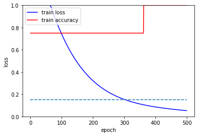
fig, loss_ax = plt.subplots()
loss_ax.plot(hist.history['loss'], 'y', label='train loss', c='blue')
loss_ax.plot(hist.history['accuracy'], 'y', label='train accuracy', c='red')
plt.plot(range(epochs), [0.15 for _ in range(epochs)], linestyle='--')
loss_ax.set_xlabel('epoch')
loss_ax.set_ylabel('loss')
loss_ax.legend(loc='upper left')
loss_ax.set_ylim(0, 1)
plt.show()
return model.predict(X)

= 눈에 띄게 좋아진것을 확인 할 수 있다.
initializer = keras.initializers.RandomNormal()
activation = 'sigmoid'
epochs = 500
optimizer = 'adam'

for _ in range(5) :
    xor_practice3(initializer, activation, epochs, optimizer)
= 낮은 epochs과 sigmoid로도 괜찮은 결과를 낼 수 있었다.
Batch Normalization
Issue : 과적합
▶ Geofferey Hinton's summary of findings up to today
- Our labeled datasets were thousands of times too small, 레이블링 데이터셋 구축
- Our computers were millions of times too slow, 병렬처리
- We initialized the weights in a stupid way, 해결
- We used the wrong type of non-linearity, 해결
▶ Dropout
Node를 On/Off한다.
너무 많은 노드는 과적합의 문제가 있다.
적은 노드로 좋은 결과를 도출한다.
* y = wx + b의 목적은 Cost function을 최소화하는 W, b를 구하는 것이다.
▶ 과적합 방지
- 데이터 양을 늘린다.
- 추가 수집, 증식, Augmentation, Back Translation 등
- Weight의 수를 줄인다.
- Regularization 적용
- L1 norm, L2 norm, L1 + L2 norm
- Dropout
▶ Sequential문
model = Sequential()
model.add(Dense(256, input_shape=(2,), activation='relu'))
model.add(Dropout(0.5))
model.add(Dense(128, input_shape=(2,), activation='relu'))
model.add(Dropout(0.5))
model.add(Dense(2, activation='softmax'))
▶ Functional문
from tensorflow.keras.layers import Dropout

xor = {'x1':[0,0,1,1], 'x2':[0,1,0,1], 'y':[0,1,1,0]}
XOR = pd.DataFrame(xor)
X = XOR.drop('y', axis=1)
y = XOR.y

initializer = initializers.RandomNormal()
ip = Input(shape=(2,))
n = Dropout(0.5)(ip)
n = Dense(2, activation='sigmoid')(n)
n = Dropout(0.5)(n)
n = Dense(1, activation='linear')(n)
model = Model(inputs=ip, outputs=n)
model.compile(loss='mse', optimizer=optimizer, metrics='accuracy')
hist = model.fit(X, y, epochs=epochs, verbose=0)'Python' 카테고리의 다른 글
| [Python] Titanic Deep Learning (0) | 2022.12.19 |
|---|---|
| [Python] K-means Algorithm (0) | 2022.11.17 |
| [Python] PCA, LDA (0) | 2022.11.17 |
| [Python] openCV : Matching (0) | 2022.11.17 |
| [Python] openCV : Moments (0) | 2022.11.17 |